2018/5/19にPycon Osakaで'librosaで始める音楽情報処理'というタイトルで発表しました
2018/5/19にPyCon mini Osakaで「librosaで始める音楽情報検索」というタイトルで発表しました
公開が遅くなりましたが先月開催されたPyCon mini Osakaで発表した内容を公開します。この記事もAzure Notebooksで既に公開済ではありましたが、nikolaのipynb公開機能を使ってブログポストとして投稿しておきたいと思います。
In [1]:
from IPython.display import IFrame
IFrame("https://www.hiromasa.info/slide/5.slides.html", "100%", "450px")
Out[1]:
librosaで始める音楽情報検索
- 大橋 宏正(twitter: @wrist)
この資料
- Azure Notebooksで作成
自己紹介
- 大橋宏正(@wrist)
- 某メーカで音響信号処理の業務に従事
- 2013年ごろから大阪PRML読書会を主催(現在休止中)
- PyData Osakaオーガナイザ
PyCon mini Osakaのテーマ
- 「Pythonでなにしよう?」
- Webアプリ
- 科学技術計算
- Pythonで音楽の分析を行いたい!
この発表
- Pythonで音楽情報検索(MIR)を行うためのライブラリlibrosaの紹介
音楽情報検索(MIR)とは?
- Music Information Retrievalの略
- 音楽情報に関する処理全般
- ビートトラッキング、楽器音分離、音楽推薦など
- コミュニティ
- ismir.net
- 音楽情報科学研究会(www.sigmus.jp)
MIRをPythonで行う
- Pythonで音楽データの処理が必要
- 読み書き
- wave, audioread, pysoundfile, scipy.io, ...
- 線形代数、信号処理、フーリエ変換
- numpy, scipy(signal, fftpack, ...)
- 可視化
- matplotlib, seaborn
- これらを組み合わせることでさまざまな処理を実現
librosa
- 音楽情報処理を行うためのPythonライブラリ
- コロンビア大学にかつて存在したLabROSAで開発
- 2/17に0.6.0がリリース
- github
- ドキュメント
librosaの特徴
- MIRに必要となる典型的な処理が多く実装
- 低い学習障壁
- 一貫性、後方互換性、モジュール性
In [1]:
# pipでインストール
!pip install librosa
librosaの具体的な紹介
- 適宜デモを交えながらlibrosaを紹介
- 発表の流れ
- 音データの短時間周波数分析
- 特徴量抽出
- オンセット検出、ビートトラッキング
In [2]:
# 本発表では以下を仮定
import numpy as np
import scipy as sp
import scipy.signal as sg
import scipy.fftpack as fft
import matplotlib as mpl
import matplotlib.pyplot as plt
import IPython.display
In [3]:
# version
print("numpy version", np.version.full_version)
print("scipy version", sp.version.full_version)
print("matplotlib version", mpl.__version__)
In [4]:
# librosa以下の各モジュールをimport
import librosa
import librosa.display
import librosa.feature
import librosa.effects
import librosa.onset
import librosa.beat
サウンドデータの読み込み
-
librosa.load- ファイルパスを与えることでデータを読み込み
- デフォルトでモノラル化、サンプリングレート22050Hzとなる
- バックエンドに
audioreadライブラリを使用
-
librosa.display.waveplotで波形データの可視化
In [5]:
# デモ音源のロード&再生
# y: モノラル音声データ, sr: サンプリングレート
y, sr = librosa.load(librosa.util.example_audio_file())
IPython.display.Audio(data=y, rate=sr)
Out[5]:
In [6]:
# 波形の描画
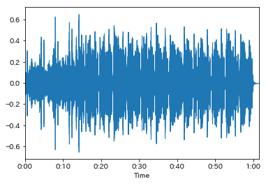
# 縦軸レンジを自動的に指定し、横軸を秒数表示にしてくれる
librosa.display.waveplot(y, sr)
Out[6]:
サウンドデータのデジタル表現
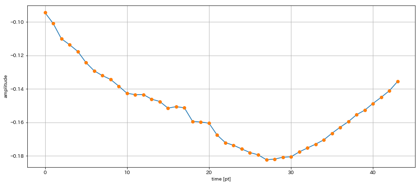
- 現実の音はアナログデータ
- 時間方向にも振幅方向にも連続
- コンピュータで音を取り扱うためには離散化が必要
- 時間方向: サンプリング
- 振幅方向: 量子化
In [7]:
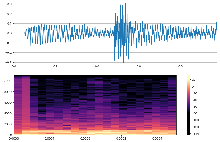
b_pt = int(10.0*sr); e_pt = int((10.0+0.002)*sr)
fig = plt.figure(1, figsize=(14,6)); ax = fig.add_subplot(111)
ax.plot(y[b_pt:e_pt]); ax.plot(y[b_pt:e_pt], "o"); ax.grid();
ax.set_xlabel("time [pt]"); ax.set_ylabel("amplitude")
Out[7]:
In [8]:
# サンプリングレート: 1秒辺りのサンプル数
print("sampling rate: {0}".format(sr))
print("length: {0}[pt]={1}[s]".format(y.shape[0], y.shape[0]/sr))
音声データの周波数分析
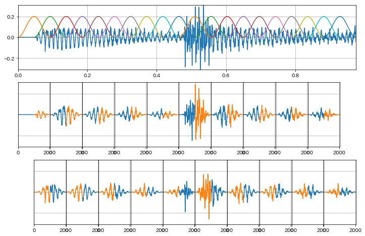
- 音声データの長さはデータにより異なる
- 固定長の短時間波形に切り出した上で処理を行う
- 短時間波形に対し離散フーリエ変換を適用することで周波数分析を行う
In [9]:
# strideトリックを使った信号を短時間波形フレームの配列に変換する関数
from numpy.lib.stride_tricks import as_strided

def split_frames(xs, frame_width=1024, noverlap=2):

    nsample = np.alen(xs)
    nshift = (frame_width // noverlap)
    nframe = int(nsample / nshift) - noverlap + 1

    nbyte = xs.dtype.itemsize

    # as_strided(xs, ys_shape, new_stride)
    xs_split = as_strided(xs, (nframe, frame_width), (nbyte * nshift, nbyte))

    return xs_split
In [10]:
def plot_overlap_waves():
    import matplotlib.gridspec as gridspec

    frame_width = 2048
    half_width = int(frame_width // 2)
    nframes = 20

    fig = plt.figure(1, figsize=(12,8))
    gs = gridspec.GridSpec(3, nframes + 1)

    ax_wav = fig.add_subplot(gs[0, :])
    ax_wav.plot(np.arange(half_width*(nframes+1))/sr,
                y[:half_width*(nframes+1)])
    ymax = np.max(y[:half_width*(nframes+1)])
    ax_wav.set_xlim([0, half_width*(nframes+1)/sr])
    ax_wav.set_ylim([-ymax, ymax]); ax_wav.grid()

    win = sg.get_window("hanning", int(frame_width))
    xs = np.arange(frame_width)

    for i, y_cut in enumerate(split_frames(y, int(frame_width), 2)[:nframes]):
        y_win = win * y_cut
        ax_wav.plot(np.arange(half_width*i, half_width*i + frame_width)/sr, 0.2 * win)
        ax = None
        if i % 2 == 0:
            ax = fig.add_subplot(gs[1, i:i+2])
            ax.plot(xs[:half_width], y_win[:half_width])
            ax.plot(xs[half_width:], y_win[half_width:])
            ax.set_xlim([0, frame_width])
        else:
            ax = fig.add_subplot(gs[2, i:i+2])
            ax.plot(xs[half_width:], y_win[half_width:])
            ax.plot(xs[:half_width], y_win[:half_width])
            ax.set_xlim([0, frame_width])

        ax.tick_params(labelleft="off",left="off") # y軸の削除
        ax.set_ylim([-ymax, ymax]); ax.grid()

    fig.subplots_adjust(wspace=0.0)
In [11]:
# 周波数分析時には通常窓関数を乗算した短時間波形を使用
# 切り出しはここでは1/2区間をオーバーラップさせている
plot_overlap_waves()
用語の整理
-
sr= sampling rate [Hz = pt/s]- 22050 [Hz]
-
frame= 各短時間波形 -
n_fft= 各フレームに含まれるサンプル数- 2048 [pt]
-
hop_length= フレーム間のサンプル数- 512 [pt]
In [12]:
def plot_overlap_freqs():
    import matplotlib.gridspec as gridspec

    frame_width = 2048
    half_width = int(frame_width // 2)
    nframes = 20

    fig = plt.figure(1, figsize=(12,8))
    gs = gridspec.GridSpec(3, nframes + 1)

    ax_wav = fig.add_subplot(gs[0, :])
    ax_wav.plot(y[:half_width*(nframes+1)])
    ymax = np.max(y[:half_width*(nframes+1)])
    ax_wav.set_xlim([0, half_width*(nframes+1)])
    ax_wav.set_ylim([-ymax, ymax]); ax_wav.grid()

    win = sg.get_window("hanning", int(frame_width))
    xs = np.arange(frame_width)
    w = np.linspace(0.0, 2.0 * np.pi, frame_width, endpoint=False)
    freqs = w[:frame_width//2+1] * (sr / 2) / np.pi
    for i, y_cut in enumerate(split_frames(y, int(frame_width), 2)[:20]):
        y_win = win * y_cut
        Y_abs = np.abs(fft.fft(y_win, frame_width)[:frame_width//2+1])
        ax_wav.plot(np.arange(half_width*i, half_width*i + frame_width), 0.2 * win)
        ax = None
        if i % 2 == 0:
            ax = fig.add_subplot(gs[1, i:i+2])
            ax.semilogy(Y_abs, freqs)
        else:
            ax = fig.add_subplot(gs[2, i:i+2])
            ax.semilogy(Y_abs, freqs)

        if i > 1:
            ax.tick_params(labelleft="off",left="off") # y軸の削除
        else:
            ax.tick_params(labelbottom="off",bottom="off") # x軸の削除
            ax.set_ylabel("frequency [Hz]")

        ax.set_xlabel("amplitude")
        ax.set_ylim([10, sr/2])
        ax.grid()

    fig.subplots_adjust(wspace=0.0)
In [13]:
# 各短時間波形を周波数分析したグラフを描画
# 縦軸が周波数、横軸が振幅スペクトル
plot_overlap_freqs()
In [14]:
def plot_spectrogram():
    frame_width = 2048
    half_width = int(frame_width // 2)
    nframes = 20

    fig = plt.figure(1, figsize=(12,8))

    ax_wav = fig.add_subplot(211)
    ax_wav.plot(np.arange(half_width*(nframes+1))/sr,
                y[:half_width*(nframes+1)])
    ymax = np.max(y[:half_width*(nframes+1)])
    ax_wav.set_xlim([0, half_width*(nframes+1)/sr])
    ax_wav.set_ylim([-ymax, ymax]); ax_wav.grid()

    win = sg.get_window("hanning", int(frame_width))
    xs = np.arange(frame_width)
    w = np.linspace(0.0, 2.0 * np.pi, frame_width, endpoint=False)
    freqs = w[:frame_width//2+1] * (sr / 2) / np.pi

    Zs = []
    for i, y_cut in enumerate(split_frames(y, int(frame_width), 2)[:20]):
        y_win = win * y_cut
        Y_abs = np.abs(fft.fft(y_win, frame_width)[:frame_width//2+1])
        ax_wav.plot(np.arange(half_width*i, half_width*i + frame_width), 0.2 * win)
        Zs.append(20.0*np.log10(Y_abs))

    ax = fig.add_subplot(212)
    Xs = np.arange((nframes+1)) / sr / 2
    pcol = ax.pcolormesh(Xs, freqs, np.array(Zs).T, cmap='magma')
    cax = fig.colorbar(pcol)
    cax.set_clim(-80, 20)

    fig.subplots_adjust(wspace=0.0)
In [15]:
# 短時間波形を周波数分析したものをスペクトログラムとして表示
plot_spectrogram()
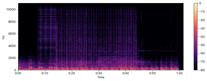
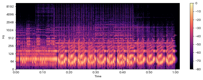
librosaにおける短時間周波数分析
- 短時間離散フーリエ変換(Short time fourie transform)
librosa.stft
- Constant-Q Transform(CQT)
librosa.cqt
- 分析結果の可視化
librosa.specshow
In [16]:
# librosaでは短時間波形分析をメソッド一発で実行可能
D = librosa.stft(y)
In [17]:
# D[k, l]
# k: 周波数ビン  l: フレームインデックス
# kは実信号に対する2048ptフーリエ変換の結果なので1025ptのみ保持
D.shape
Out[17]:
離散フーリエ変換$D[k,l]$の算出法
$$D[k, l]=\sum_{n=0}^{{\textrm N_{\rm fft}-1}} w[n]\cdot x\left[\left(l\cdot {\rm M}-\frac{N_{\rm fft}}{2}\right)+n\right]\exp\left\{-j\frac{2\pi k n}{N_{\rm fft}}\right\}$$* $x[n]$は入力信号、$w[n]$は窓関数
* 周波数ビン$k$、フレームインデックス$l$、$M$はhop length
* $lM$を中心に前後$N/2$点に渡り離散フーリエ変換を実行In [18]:
fig = plt.figure(1, figsize=(12,4)); ax = fig.add_subplot(1,1,1)

log_power = librosa.amplitude_to_db(np.abs(D), ref=np.max)
librosa.display.specshow(log_power, x_axis="time", y_axis="linear")
plt.colorbar()
Out[18]:
In [19]:
# 縦軸を対数表示
fig = plt.figure(1, figsize=(12,4)); ax = fig.add_subplot(1,1,1)

log_power = librosa.amplitude_to_db(np.abs(D), ref=np.max)
librosa.display.specshow(log_power, x_axis="time", y_axis="log")
plt.colorbar()
Out[19]:
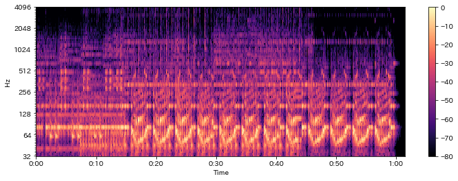
Constant-Q変換
$$C[k]= \frac{1}{N[k]} \sum_{n=0}^{{\textrm N[k]-1}} w[n, k]\cdot x\left[n\right]\exp\left\{-j\frac{2\pi Q[k] n}{N[k]}\right\}$$- 特徴
- 分析する周波数間隔を対数的に配置
- 低域は細かく分析し、高域は荒く分析
- 音楽信号の分析に適する
In [20]:
C = librosa.cqt(y, sr)
In [21]:
# STFTと比較して縦軸の周波数データ数は圧倒的に少ない
# STFTは周波数間隔が等幅なのに対してCQTだと対数間隔となるため
print(D.shape)
print(C.shape)
In [22]:
fmin = 32.70  # C1に相当するHz
fmax = fmin * ((2**(1/12)) ** 84)
print(fmax)
print(librosa.hz_to_note(fmin))
print(librosa.hz_to_note(fmax))
In [23]:
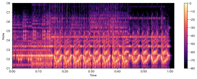
fig = plt.figure(1, figsize=(12,4)); ax = fig.add_subplot(1,1,1)

log_cqt_power = librosa.amplitude_to_db(np.abs(C), ref=np.max)
librosa.display.specshow(log_cqt_power, x_axis="time", y_axis="cqt_hz")
plt.colorbar()
Out[23]:
In [24]:
fig = plt.figure(1, figsize=(12,4)); ax = fig.add_subplot(1,1,1)

log_cqt_power = librosa.amplitude_to_db(np.abs(C), ref=np.max)
librosa.display.specshow(log_cqt_power, x_axis="time", y_axis="cqt_note")
plt.colorbar()
Out[24]:
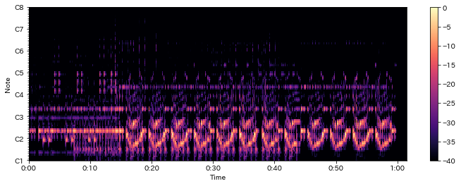
In [25]:
fig = plt.figure(1, figsize=(12,4)); ax = fig.add_subplot(1,1,1)

# デフォルトだと80dBまでだがtop_dbを付けるとレンジが縮まる
log_cqt_power = librosa.amplitude_to_db(np.abs(C), ref=np.max, top_db=40)
librosa.display.specshow(log_cqt_power, x_axis="time", y_axis="cqt_note")
plt.colorbar()
Out[25]:
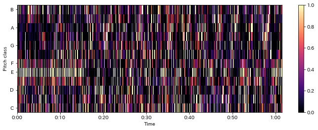
クロマベクトル
- 12音階それぞれの強さを要素に持つベクトル
- CQTで算出した対数周波数帯域ごとの強度を元に計算
librosa.feature.chroma_cqt
In [26]:
chroma = librosa.feature.chroma_cqt(C=C, sr=sr)

fig = plt.figure(1, figsize=(12,4)); ax = fig.add_subplot(1,1,1)

librosa.display.specshow(chroma, x_axis="time", y_axis="chroma")
plt.colorbar()
Out[26]:
In [27]:
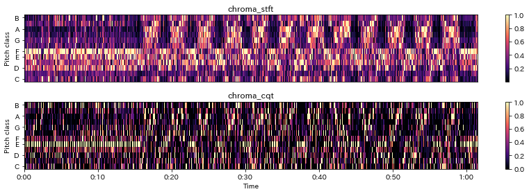
# STFTの結果Dからクロマベクトルを算出
chroma_stft = librosa.feature.chroma_stft(S=D, sr=sr)

fig = plt.figure(1, figsize=(12,4))
ax = fig.add_subplot(2,1,1)
librosa.display.specshow(chroma_stft, y_axis='chroma')
plt.title('chroma_stft'); plt.colorbar()
ax= fig.add_subplot(2,1,2)
librosa.display.specshow(chroma, y_axis='chroma', x_axis='time')
plt.title('chroma_cqt'); plt.colorbar()
plt.tight_layout()
その他特徴量抽出
- メルスペクトル、MFCC、tonnetzなども算出可能
- $\Delta$特徴量の計算も可能
In [28]:
M = librosa.feature.melspectrogram(y=y, sr=sr)
mfcc = librosa.feature.mfcc(y=y, sr=sr)
tonnetz = librosa.feature.tonnetz(y=y, sr=sr)
librosa.effectsモジュール
- 音源分離
-
librosa.hpss- 調波成分と打音成分に分解
-
- 時間伸縮、ピッチシフト
librosa.time_stretchlibrosa.pitch_shift
In [29]:
y_harmonic, y_percussive = librosa.effects.hpss(y)
In [30]:
IPython.display.Audio(y, rate=sr)
Out[30]:
In [31]:
IPython.display.Audio(y_harmonic, rate=sr)
Out[31]:
In [32]:
IPython.display.Audio(y_percussive, rate=sr)
Out[32]:
In [33]:
# それぞれに対するCQTを求める
C      = librosa.cqt(y=y, sr=sr)
C_harm = librosa.cqt(y=y_harmonic, sr=sr)
C_perc = librosa.cqt(y=y_percussive, sr=sr)
In [34]:
fig = plt.figure(1, figsize=(12,4)); ax = fig.add_subplot(1,1,1)
log_cqt_power= librosa.amplitude_to_db(np.abs(C), ref=np.max)
log_cqt_harm = librosa.amplitude_to_db(np.abs(C_harm), ref=np.max(np.abs(C)))
log_cqt_perc = librosa.amplitude_to_db(np.abs(C_perc), ref=np.max(np.abs(C)))
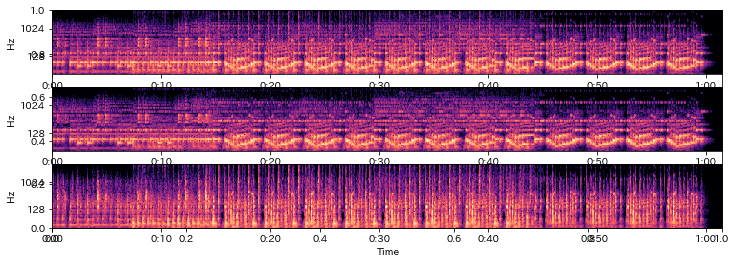
ax = fig.add_subplot(3,1,1); librosa.display.specshow(log_cqt_power, x_axis="time", y_axis="cqt_hz")
ax = fig.add_subplot(3,1,2); librosa.display.specshow(log_cqt_harm , x_axis="time", y_axis="cqt_hz")
ax = fig.add_subplot(3,1,3); librosa.display.specshow(log_cqt_perc , x_axis="time", y_axis="cqt_hz")
Out[34]:
In [35]:
# 2倍の速度に時間伸縮
y_fast = librosa.effects.time_stretch(y, 2.0)
IPython.display.Audio(y_fast, rate=sr)
Out[35]:
In [36]:
# 3度上にピッチシフト
y_third = librosa.effects.pitch_shift(y, sr, n_steps=4)
IPython.display.Audio(y_third, rate=sr)
Out[36]:
In [37]:
# 減五度にピッチシフト
y_tritone = librosa.effects.pitch_shift(y, sr, n_steps=-6)
IPython.display.Audio(y_tritone, rate=sr)
Out[37]:
onset検出とビートトラッキング
-
librosa.onsetモジュール、librosa.beatモジュールを使用- 出音の強度を
onset.onset_strengthで算出 - 強度を元にonset箇所を
onset.onset_detectで検出 - 強度を元に
beat.beat_trackでテンポとビートを推定
- 出音の強度を
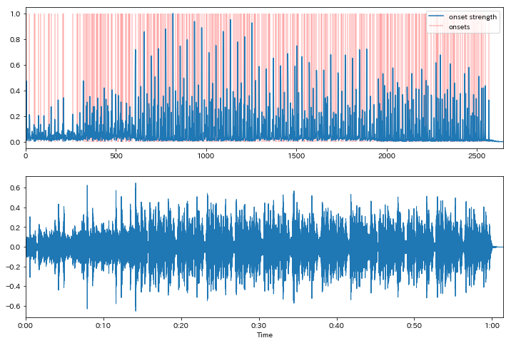
In [38]:
onset_envelope = librosa.onset.onset_strength(y, sr)
onsets = librosa.onset.onset_detect(onset_envelope=onset_envelope)
In [39]:
fig = plt.figure(1, figsize=(12,8))
ax = fig.add_subplot(2, 1, 1)
ax.plot(onset_envelope, label="onset strength")
ax.vlines(onsets, 0, np.max(onset_envelope), color="red", alpha=0.25, label="onsets")
ax.set_xlim([0, len(onset_envelope)]); ax.legend(loc=1)
ax = fig.add_subplot(2, 1, 2)
librosa.display.waveplot(y, sr)
Out[39]:
In [40]:
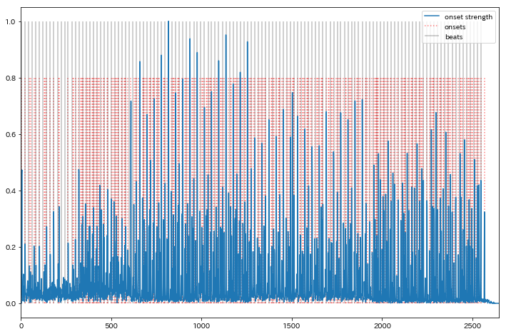
tempo, beats = librosa.beat.beat_track(onset_envelope=onset_envelope)
In [41]:
print(tempo)
In [42]:
fig = plt.figure(1, figsize=(12,8))
ax = fig.add_subplot(1, 1, 1)
ax.plot(onset_envelope, label="onset strength")
ax.vlines(onsets, 0, 0.8 * np.max(onset_envelope), color="red", alpha=0.5, linestyle="dotted", label="onsets")
ax.vlines(beats, 0, np.max(onset_envelope), color="black", alpha=0.25, label="beats")
ax.set_xlim([0, len(onset_envelope)]); ax.legend(loc=1)
Out[42]:
クリック音を生成し同時に再生
- MIRの評価に用いられる
mir_evalライブラリを使用
In [43]:
!pip install mir_eval
In [44]:
# http://colinraffel.com/publications/ismir2014mir_eval.pdf
import mir_eval
In [45]:
beat_times = librosa.frames_to_time(beats)
y_click = mir_eval.sonify.clicks(beat_times, sr, length=len(y))
In [46]:
IPython.display.Audio(y_click, rate=sr)
Out[46]:
In [47]:
IPython.display.Audio(y + y_click, rate=sr)
Out[47]:
特徴量のビート同期
-
librosa.util.syncを用いるとビートとその他特徴量を同期させることができる- 各ビートの間の成分を平均化したり中央値を取ったりできる
In [48]:
tempo, beat_frames = librosa.beat.beat_track(y=y_percussive, sr=sr)
# 13次元のMFCCおよびΔを抽出
mfcc = librosa.feature.mfcc(y=y, sr=sr, n_mfcc=13)
mfcc_delta = librosa.feature.delta(mfcc)
In [49]:
print(beat_frames.shape)
print(mfcc.shape)
print(mfcc_delta.shape)
In [50]:
# ビート間の平均値を用いてMFCCとΔMFCCをビートに同期
beat_mfcc_delta = librosa.util.sync(np.vstack([mfcc, mfcc_delta]),
                                    beat_frames)
In [51]:
beat_mfcc_delta.shape
Out[51]:
In [52]:
# 調波成分からクロマベクトルを推定
chromagram = librosa.feature.chroma_cqt(y=y_harmonic, sr=sr)

# ビート間の中央値を用いてクロマベクトルをビートに同期
beat_chroma = librosa.util.sync(chromagram, beat_frames, aggregate=np.median)

# ビート同期特徴量(クロマベクトル、MFCC、ΔMFCC)を結合
beat_features = np.vstack([beat_chroma, beat_mfcc_delta])
In [53]:
# MFCC 13dim, ΔMFCC 13dim, クロマベクトル(12音階; 12dim)
beat_features.shape
Out[53]:
In [54]:
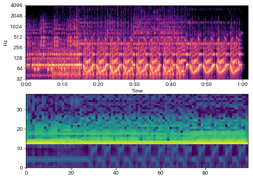
fig = plt.figure(figsize=(8,6))
ax = fig.add_subplot(211)
librosa.display.specshow(log_cqt_power, x_axis="time", y_axis="cqt_hz")
log_beat_features = librosa.amplitude_to_db(np.abs(beat_features), ref=np.max)
ax = fig.add_subplot(212)
ax.pcolormesh(log_beat_features)
Out[54]:
まとめ
- librosaを用いた音楽情報検索(MIR)について説明
- 特徴量抽出、可視化、音源分離、ビート推定
- 音楽データに対する探索的分析の手段の一つ
以下補足およびおまけ
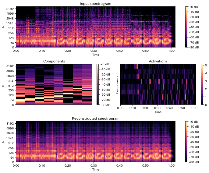
librosa.decomposeによる音源分離
- NMFによるモノラル音源分離を行う
- スペクトログラムを行列と見て
scikit-learnのNMFに投げる - アクティベーション行列と基底行列に分解
- 教師なし音源分離が可能
- スペクトログラムを行列と見て
NMF
- 非負値行列$\textbf{X}$を$\textbf{X} \simeq \textbf{WH} $と分解する手法
- Hを基底行列、Wをアクティベーションと呼ぶ
- scikit-learnのNMFでは下記目的関数を最小化
- 通常最適化には補助関数法が使われる
In [55]:
D = librosa.stft(y)
S, phase = librosa.magphase(D)
comps, acts = librosa.decompose.decompose(S, n_components=8, sort=True)
S_approx = comps @ acts
In [56]:
print(comps.shape)
print(acts.shape)
print(S.shape, S_approx.shape)
In [57]:
def plot_decomposed(S, comps, acts, S_approx):
    fig = plt.figure(figsize=(10,8))
    ax = fig.add_subplot(311)
    librosa.display.specshow(librosa.amplitude_to_db(S, ref=np.max), y_axis='log', x_axis='time')
    ax.set_title('Input spectrogram'); plt.colorbar(format='%+2.0f dB')

    ax = fig.add_subplot(323)
    librosa.display.specshow(librosa.amplitude_to_db(comps, ref=np.max), y_axis='log')
    plt.colorbar(format='%+2.0f dB'); ax.set_title('Components')

    ax = fig.add_subplot(324)
    librosa.display.specshow(acts, x_axis='time')
    ax.set_ylabel('Components'); ax.set_title('Activations')
    plt.colorbar()

    ax = fig.add_subplot(313)
    librosa.display.specshow(librosa.amplitude_to_db(S_approx, ref=np.max), y_axis='log', x_axis='time')
    plt.colorbar(format='%+2.0f dB')
    ax.set_title('Reconstructed spectrogram')

    fig.tight_layout()
In [58]:
plot_decomposed(S, comps, acts, S_approx)
In [59]:
S_partly = comps[:, :3] @ acts[:3, :]
In [60]:
plot_decomposed(S, comps[:, :3], acts[:3, :], S_partly)
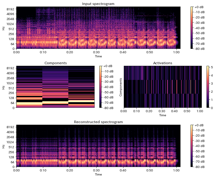
In [61]:
y_partly = librosa.istft(S_partly * phase)
IPython.display.Audio(y_partly, rate=sr)
Out[61]:
decomposeの用途
- 視聴用途の音源分離には(このままでは)向かない
- 振幅スペクトルのみを分解するが、位相情報は元信号の元を使うため歪が大きい
- 基底数を増加した上で適切なクラスタリングを施して使用したり、事前学習した楽器別の基底などを用いて分離を行うなどの工夫が必要
- 音響イベント検出のための特徴量に用いることも可能
コメント
Comments powered by Disqus